
How were these maps made?
We hope it will give you a good understanding of the unique process we’ve developed to create our maps. For detailed information on our workflow, please read our paper in Nature Scientific Reports.
Our key output is spatial predictions of crucial soil nutrients and properties, based on the predictive soil mapping (PSM) techniques. The first step in this process is to standardise all the input soil data by i) ensuring all measured units are in the same format; ii) harmonizing properties measured using different techniques; and iii) removing any erroneous datapoints.
An extensive selection of covariates is then used to predict soil properties across Africa. We apply a multiscale ensemble machine learning approach that combines input covariates at two different geospatial resolutions:
- Coarse scale: 250m (includes climatic and vegetation variables based on MODIS satellite products and similar)
- Fine scale: 30m (includes digital terrain model (DTM) derivatives, as well as Sentinel-2 satellite and and Landsat-7/8 cloud-free composite images)
We then apply five regression modelling algorithms:
- Random forest as implemented in the Ranger package
- Gradient boosting as implemented in the XGBoost package
- Cubist regression models as implemented in the Cubist package
- Neural network algorithms as implemented in the deepnet package
- GLM with Lasso or Elasticnet Regularization as implemented in the glmnet package
All programming has been implemented in the R software for statistical computing, using open source packages and applications for spatial analysis. For each property, we run model fine tuning, feature selection (to reduce the number of covariates) and ensemble machine learning, using the SuperLearner algorithm as implemented in the mlr package.
Predictions at the coarse (250m) and fine (30m) resolutions are generated independently, then merged using ensembling. We first predict values at three depths: 0, 20cm and 50cm, then aggregate values to standard depth intervals (0–20cm and 20–50cm). In principle, all steps — apart from the soil data import and feature selection — are fully automated and assume no human interaction.
Computing is implemented in a high performance system with tasks fully parallelized using the R snowfall package. The overall workflow is outlined in the schematic below.
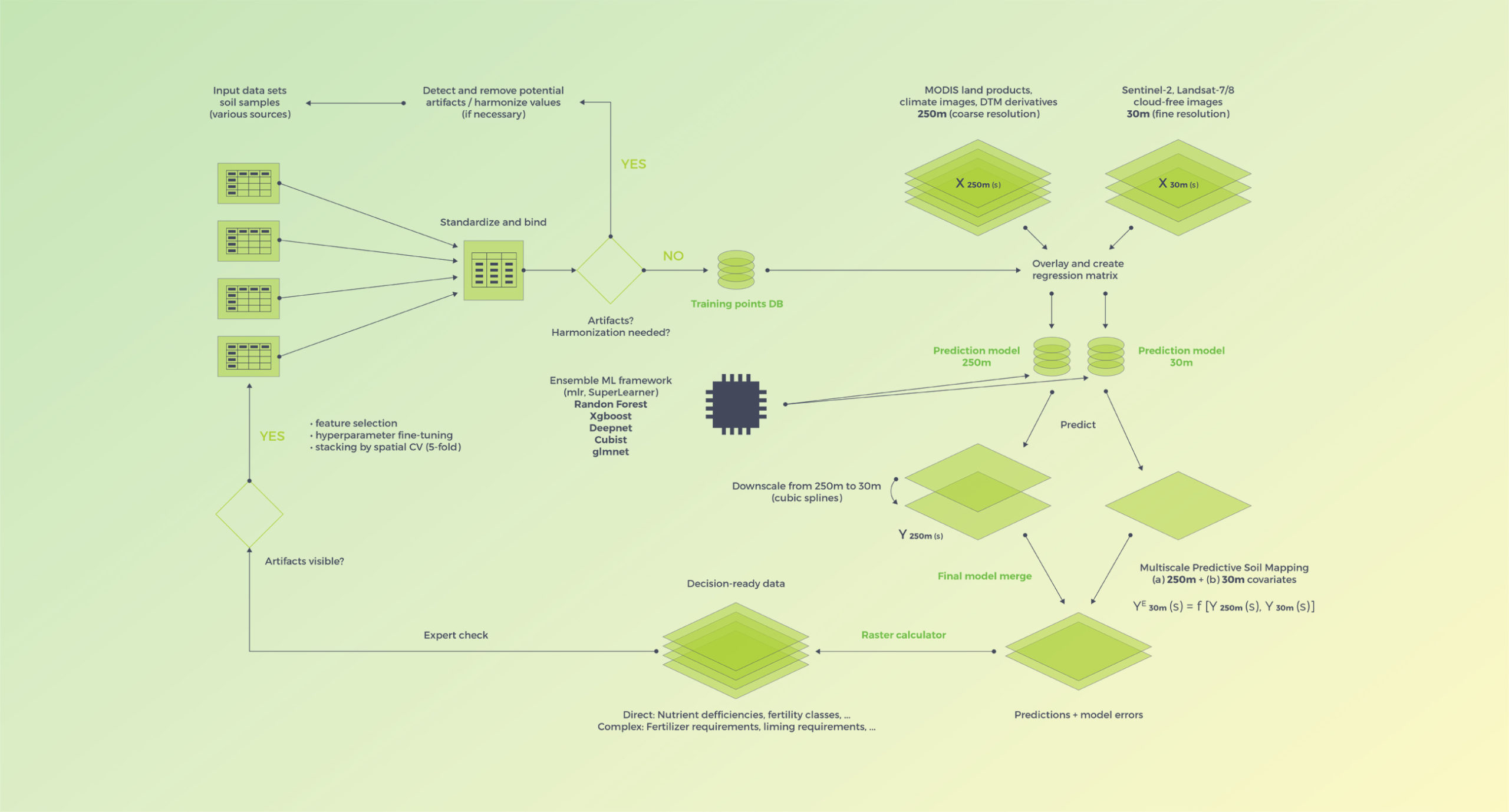
General computational scheme using a 2-scale system (250m and 30m covariates) and ensemble machine learning based on the mlr R framework for machine learning
As training points we have used a compilation of legacy soil profiles and point data from various datasets. The total number of training points used depends on the soil property, but is generally higher than 100,000.
Important point datasets include:
- AfSIS I and II soil samples for Tanzania, Uganda, Nigeria, Ghana: ~ 40,000 sampling locations, based upon spectral and wet chemistry data. AfSIS I dataset prepared by ICRAF: https://doi.org/10.34725/DVN/QXCWP1
- ISRIC Africa Soil Profile Database: ~ 13,000 legacy profiles collected across Africa and collated by ISRIC as part of the AfSIS project
- LandPKS: ~ 12,000 soil profile observations, crowd sourced and collected via the LandPKS mobile app
- IFDC: ~ 9,000 soil sampling locations across Ghana, Uganda, Rwanda and Burundi collected from various projects
- AfricaRice and TAMASA: > 3,000 soil sampling locations across Africa generated from field trials by AfricaRice and Taking Maize Agronomy to Scale in Africa (TAMASA)
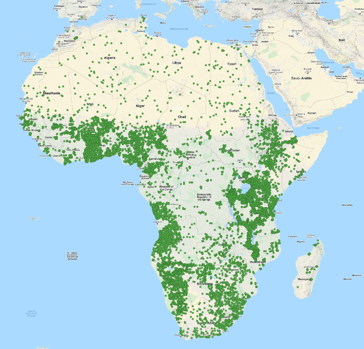
Locations of training points used in iSDAsoil
The iSDAsoil predictions are a major update of the predictions published in 2017 by Hengl et al. There are two key methodological differences between the 2017 predictions and those we’ve produced:
- We’ve increased the target spatial resolution of our predictions from 250m to 30m, making the data volume 60–100 times larger.
- The level of detail for soil property predictions is significantly improved by adding Sentinel-2 and Landsat-7/8 cloud-free satellite images. These were derived using Amazon AWS Sentinel and Landsat services for seasons 2018 and 2019.
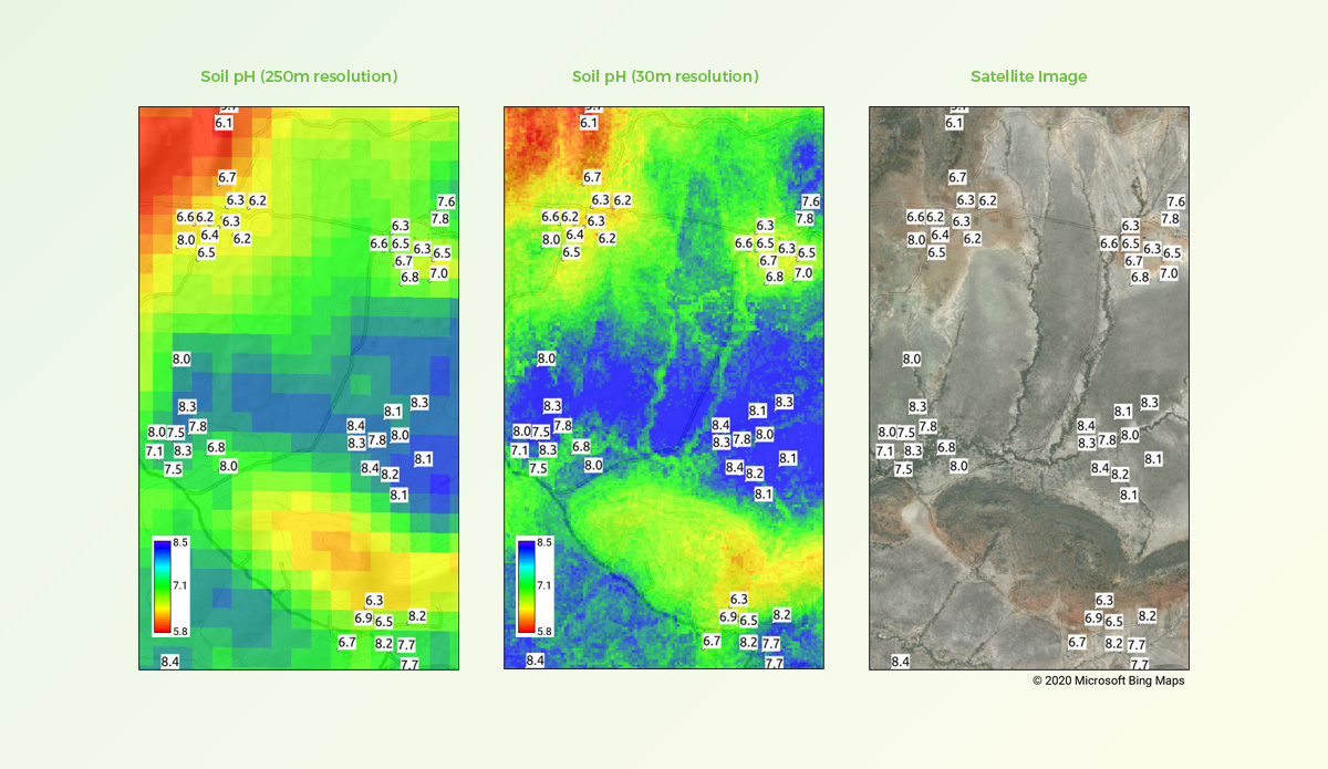
Comparison of soil pH predictions at 250m and 30m spatial resolutions
Left: predicted pH results using standard 250m resolution. Centre: results using 30m resolution as developed for iSDAsoil. Right: satellite image showing geographical features of this location. Labels indicate measured pH values based on soil samples collected from the field.
Improvements in both spatial accuracy and detail are reflected in the accompanying maps for a location in Kenya, where soil samples used in our model training had been collected. We were pleased to find that our predicted data for this location were a good match with features in the field, as well as with our original training data.
We can also report two other kinds of improvement. One concerns the accuracy of our mapping system (using 5-fold spatial block-cross-validation with refitting). The other is our ability to provide a measure of uncertainty alongside each data point, derived as the model variance from the significant learners.
We continue to work on current limitations, such as soil properties that remain challenging to map. Nevertheless, we’re proud of the progress our team has made to date, and we look forward to sharing new developments with the community as they arise. If you have technical or other questions related to our mapping, visit our FAQs or drop us a line.